PDF Publication Title:
Text from PDF Page: 021
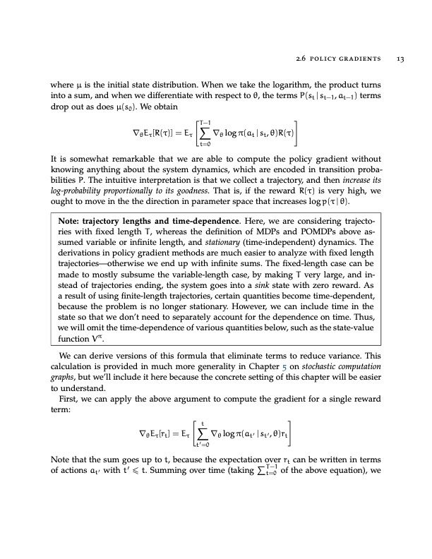
2.6 policy gradients 13 where μ is the initial state distribution. When we take the logarithm, the product turns into a sum, and when we differentiate with respect to θ, the terms P(st | st−1, at−1) terms drop out as does μ(s0). We obtain T−1 ∇θ log π(at | st, θ)R(τ) It is somewhat remarkable that we are able to compute the policy gradient without knowing anything about the system dynamics, which are encoded in transition proba- bilities P. The intuitive interpretation is that we collect a trajectory, and then increase its log-probability proportionally to its goodness. That is, if the reward R(τ) is very high, we ought to move in the the direction in parameter space that increases log p(τ | θ). ∇θEτ[R(τ)] = Eτ t=0 Note: trajectory lengths and time-dependence. Here, we are considering trajecto- ries with fixed length T, whereas the definition of MDPs and POMDPs above as- sumed variable or infinite length, and stationary (time-independent) dynamics. The derivations in policy gradient methods are much easier to analyze with fixed length trajectories—otherwise we end up with infinite sums. The fixed-length case can be made to mostly subsume the variable-length case, by making T very large, and in- stead of trajectories ending, the system goes into a sink state with zero reward. As a result of using finite-length trajectories, certain quantities become time-dependent, because the problem is no longer stationary. However, we can include time in the state so that we don’t need to separately account for the dependence on time. Thus, we will omit the time-dependence of various quantities below, such as the state-value function Vπ. We can derive versions of this formula that eliminate terms to reduce variance. This calculation is provided in much more generality in Chapter 5 on stochastic computation graphs, but we’ll include it here because the concrete setting of this chapter will be easier to understand. First, we can apply the above argument to compute the gradient for a single reward term: t ∇θ logπ(at′ |st′,θ)rt ∇θEτ[rt] = Eτ Note that the sum goes up to t, because the expectation over rt can be written in terms t′=0 of actions a ′ with t′ t. Summing over time (taking T−1 of the above equation), we t t=0PDF Image | OPTIMIZING EXPECTATIONS: FROM DEEP REINFORCEMENT LEARNING TO STOCHASTIC COMPUTATION GRAPHS

PDF Search Title:
OPTIMIZING EXPECTATIONS: FROM DEEP REINFORCEMENT LEARNING TO STOCHASTIC COMPUTATION GRAPHSOriginal File Name Searched:
thesis-optimizing-deep-learning.pdfDIY PDF Search: Google It | Yahoo | Bing
Cruise Ship Reviews | Luxury Resort | Jet | Yacht | and Travel Tech More Info
Cruising Review Topics and Articles More Info
Software based on Filemaker for the travel industry More Info
The Burgenstock Resort: Reviews on CruisingReview website... More Info
Resort Reviews: World Class resorts... More Info
The Riffelalp Resort: Reviews on CruisingReview website... More Info
| CONTACT TEL: 608-238-6001 Email: greg@cruisingreview.com | RSS | AMP |